can you learn calculus in the time it takes to watch long movie yes you can my name is Dennis Davis I'm an engineer not mathematician try to make my videos visually enlightening and fast-paced but this video is very long because it covers almost the entire first year of calculus using visuals graphs and diagrams I'd rather show you calculus visual then just tell you the rules and formulas if you see where the rules and formulas come from that can help you understand remember and make use of them to become truly proficient at calculus you'll need practice which you won't get just by watching this video in the description I'll link to some helpful practice oriented videos by others whether you're new to calculus studying it now or just want refresher hope you'll find this video informative and engaging my only assumptions are that you're already familiar with functions and algebra so here we go calculus is the study of change and rates of change of mathematical functions when we use calculus we perform operations on functions that result in different functions this isn't new idea at all we perform operations such as addition on numbers to get new numbers we operate on sets to get new sets on matrices to get new matrices and we can operate on functions to get new functions in fact you've probably already done this in algebra when you had function and found its inverse we start with function ofx and write out in terms of and so that equals some function of then we rewrite the equation switching and then solve the second equation for and that's the inverse of the first function so we start with function perform an operation on it and get new function the point is taking an existing function and Performing some operation on it to get new function isn't new or advanced math concept and that's really what calculus is in fact calculus is all about performing two operations on functions that's it that's calculus the first operation is called differentiation when we differentiate function the new resulting function is called the derivative of the first function the derivative is the first topic we'll cover learning to take the derivative of wide variety of function types is roughly the first semester of calculus the second calculus operation is called integration when we integrate function the new resulting function is called the integral of the first function integration is roughly the second semester of calculus and there's wonderful relationship between these two operations that we'll get to at just the right time when functions are simple these operations are simple and calculus is simple it's when the functions we operate on get complex that calculus seems complex so if calculus has reputation for being difficult subject it's not really calculus fault we'll start with the derivative and consider simple function ofx = -1 this is linear function so its graph is straight line said calculus was the study of change and rates of change and the rate of change of straight line is its slope rise over run deltay over Delta like to color code things in my videos I'm using blue for coordinates and distances and yellow for and I'll use pink for slope or rates of change won't draw lot of attention to the colors and may not mention them again but their consistent use may let you see some apparent order or pattern that might not otherwise be clear for straight line it's easy to find the slope just pick any two points and subtract their and coordinates to get Delta over Delta Delta is 3 - 0 this distance the difference between the yellow y-coordinates and Delta is 4 min-1 this distance the difference between the blue coordinates so for this linear function the slope is 3 over 3 or POS 1 for every unit changes changes by one times that amount since the slope is one if the slope were positive 1/2 then when changes by some amount changes by positive 1/2 as much if the slope were -2 then when changes changes by -2 times as much that is two times as much but in the opposite direction would get smaller as gets larger when the graph line is horizontal the slope is zero because never changes so Delta is zero when the graph line is vertical the slope is undefined because never changes Delta is zero so Delta over Delta is undefined since the denominator is zero everything's nice and simple when the function is linear but what about the function FX = x^2 - 2x + 1 the graph of this function is parabola so now the question what's the slope prompts new question in response where do you mean because the slope is smoothly changing it's different at different points suppose we want to define the slope of the function at xals 1.6 here now if you know calculus or more specifically the rules of differentiation that we'll cover soon then within few seconds you can figure out that the slope at = 1.6 is 1.2 if you don't know calculus yet promise that soon you'll know how to do this but without calculus it's not easy after all slope is rise over run deltay over Delta but with just one point where does Delta come from or Delta slope is the rate of change and there's no change at single point there's only change between two points so it's tricky question we could eyeball it by drawing our best attempt at line tangent to the curve at = 1.6 then measure the slope it won't be very accurate it's not always easy to draw an accurate tangent line but without calculus that might be an option but let me show another way in the 1600s the great minds that developed calculus approach the problem this way I'll zoom in on our grid at the red point of Interest where equals 1.6 we want to know the slope at the red point warnant you like to color code things let's choose nearby Point green and find the slope deltay over Delta between red red and green so we estimate the slope at red as the slope of the pink line between red and green Delta over Delta it'll be pretty close and the closer green is to Red the better the estimate this is the approach that will lead us to the derivative the value of our red point where we want to know the slope is 1.6 we find the value by plugging 1.6 into the function and we get 0. 36 let's choose nearby value for the Green Point let's say 1.61 so we find the yvalue for the nearby Green Point by plugging 1.61 into our function to get 361 1201 remember here's our function = x^2 - 2x + 1 we can easily find the slope deltay over Delta between two points given their coordinates and we get 1.21 the slope between red and green which is our estimate for the slope at Red calculus will tell us promise that the slope at Red is 1.2 so our estimate is very close the closer we let green get to Red the closer the estimate will get to 1.2 so let's prove it we'll still choose nearby Green Point point but now instead of choosing an actual small distance away from Red such as 0.1 or .001 we'll use variable for the tiny distance to green and call it the coordinates of the red Point are still 1.6 comma 0.36 but let's consider the coordinates of the Green Point its coordinate is 1.6 + and its y-coordinate is the function's value when we plug in 1.6 + for now let's find the slope as Delta over Delta Delta is the y-coordinate of the Green Point of 1.6 + minus the y-coordinate of the red point which is still 0.36 I'm shading the components to the color of the corresponding point and Delta is the coordinate at Green 1.6 + minus the coordinate at red 1.6 the denominator Delta looks pretty easy to simplify 1.6 + - 1.6 is simply this makes sense we chose over here to be Delta so to find Delta over Delta we'll need to expand this expression by taking our function ofx and rewriting it substituting 1.6 + in for this is just algebra so I'm showing it quickly pause if you want to step through the details we end up with this expression for the yalue of the nearby Green Point so we can now find deltay over Delta 36 + 1.2 + h^ 2 -36 all over the +36 and minus. 36 cancel leaving us with 1.2 + h^2 over as long as is not zero which it's not it's some tiny tiny change but not zero then we can cancel an from each term and the slope Delta over Delta is 1.2 + let's remember that we said was an arbitrarily small number we're going to find the limit of Delta over Delta as approaches zero you may be familiar with the concept of the limit from studying discontinuous functions in algebra we write the limit like this and underneath variable right arrow and literal value we read this as the limit as approaches zero in our case the limit of 1.2 + as approaches zero as gets closer and closer to zero the expression 1.2 + gets closer and closer to 1.2 so the limit is 1.2 and that's deltay over Delta the slope at the red point or at least the slope as Delta we called it approaches zero and now we can continue our dialogue what's the slope where do you mean at = 1.6 the slope there is 1.2 that we found by taking the slope between two very close points at the limit as the difference between their coordinates approach zero want to review this equation again which is how we estimate the slope of function at point using algebra you'll see this important expression in the first chapter of every single calculus textbook we're going to use it several more times and want to make sure you're comfortable with it it's the algebra behind estimating the slope at the red Point as the slope between the red point and the nearby Green Point the Delta over Delta the difference between the y-coordinates is Delta the numerator of our slope estimate the difference between the coordinates is Delta the denominator of our slope estimate we just need to come up with expressions for these differences the coordinate of the red point is simply so the red y-coordinate is the function's value at ofx the coordinate of the nearby Green Point is + is the small Delta amount we added to to get nearby point so the green coordinate is the function's value at + of X+ so for the numerator we can plug in the difference ofx + hus ofx can include the green and red memory aid coordinate of green minus coordinate of red for the denominator we get + - green coordinate minus red coordinate well it doesn't get written out this way very often since + - so obviously simplifies to and is the small distance we deliberately chose for Delta in the first place so the denominator is usually just same thing so when you see this expression please think of this triangle and the rise overrun slope it represents Delta over Delta two quick points first I'm illustrating positive slope but if the slope were negative the expression will correctly result in negative estimate for the slope since ofx is greater than ofx + subtracting larger number from smaller will result in negative number is always positive since it's the small Delta we added to so the equation works for positive and negative slopes the second point is the key idea that uses this expression as the entryway into calculus let me make copy of the diagram and expression the top and bottom start out identical but I'm going to make changes to the bottom to transform it step by step into the key Foundation of calculus we used the limit moment ago to find that the slope of our function was 1.2 when we take the limit as Delta approaches 0 something very special happens first the nearby Green Point approaches the red Point that's pretty obvious since is the distance between their coordinates and it's approaching zero second the expression is no longer an estimate of the slope it is the slope or what we call the derivative so let me change the header the expression at the limit isn't the algebraic estimate of the slope it's the algebraic definition of the derivative and there's one more important change at the limit Delta and Delta get new names and symbols they're called Dy and DX the stands for differential we'll talk more about it soon on the top is the estimated slope of curve based on nearby points on the bottom is the definition of the derivative at the limit is the horizontal distance between the two points approaches zero so here's how we use the limit to find the derivative at 1.6 there was lot of algebra involved to get to our answer 1.2 but no calculus yet you might not believe me but you will soon calculus is easier than taking limits taking limits with algebra is tedious this is tedious certainly not difficult but timec consuming and prone to errors if you're not careful and when promised to show you how you could know almost immediately that the slope at 1.6 was 1.2 was not talking about doing all this algebra in your head calculus is easier than this and I'll show you there's just one more key step the destination will make the journey worth it so we just found the slope of the function at = 1.6 by plugging 1.6 into the function and finding the slope to nearby Green Point now let's see what happens when we generalize we'll algebraically evaluate Delta over Delta at the variable value instead of the specific value 1.6 the Delta over Delta formula has the same Parts the y-coordinate of the nearby Green Point is ofx + the y-coordinate of the red point is ofx the coordinate of the Green Point is + and the coordinate of the red point is the denominator of course simplifies to so when we expand of + we get + h^ 2 - 2 * + + 1 and you can see the correspondence to the terms in the function we just plug in + for expand and simplify using algebra so here's the coordinate of the Green Point in terms of it's the first term in the numerator of our deltay over Delta slope expression next we need to subtract ofx which is right here minus ofx three terms cancel and we're left with these terms as Delta h^2 + 2 xh - 2 the denominator is the arbitrarily small number we chose for Delta we cancel an from each term and get Delta y/ Delta = + 2x - 2 let's let take the limit as approaches we get 2x - 2 now let's pause for moment and appreciate what we've just done we have an expression for the slope of the function = x^2 - 2x + 1 in terms of have we just found function that Returns the slope of another function let's call the second function fime of and try it out more on this prime notation shortly moment ago we found that the slope at = 1.6 is 1.2 so let's try out our new general function frime of at 1.6 we get 2 * 1.6 - 2 3.2 - 2 yes we get 1.2 just like before let's try this point at the vertex of the parabola where xal 1 it looks like the slope we get should be zero frime of 1 = 2 * 1 - 2 yes it's zero and we have indeed found the function frime of that Returns the slope of ofx for any value of and now we can finish our dialogue with the broader question what's the slope of this function at any and the answer for this function is 2x - 2 because this will return the slope of x^2 - 2x + 1 for any so we've just performed the first calculus operation differentiation we started with function ofx = x^2 - 2x + 1 and we performed an operation on it to yield new function the first function's derivative fime of = 2x - 2 the derivative of function evaluates to the slope of that function at every value we found the derivative the hard way by taking limits and crunching through algebra I'll show simpler way in moment but regardless of the method we've just performed the differentiation operation to get the derivative of function since the derivative of function is just another function we can graph it also the pink line is fime of = 2x - 2 frime of is common notation for the derivative of ofx I'll cover some notation conventions in moment the pink line represents the derivative of the white Parabola so of course the derivatives value at = 1.6 is 1.2 the slope of the parabola at = 1.6 let's go over some vocabulary and notation concerning derivatives with slopes we quite naturally speak of Delta over Delta the slope between two points this ratio gets closer and closer to the slope at as Delta gets closer and closer to zero in calculus we introduced new terms for Delta and Delta that have the limit as Delta approaches zero concept built in we say that the limit as Delta approaches zero of Delta is DX we use lowercase instead of the Greek letter Delta as calculus shorthand that means at the limit so when you see it means means at the limit as the change to the independent variable often approaches zero one more time instead of writing all this you can just write this which means the same thing it's common to think of DX as the slightest tiniest change in and this thought might serve you well but DX is really whatever Delta becomes as it gets closer and closer to zero it's an idea that we treat like number DX is called the different differential of I'll have to draw it with some sort of thickness so we can see it but it's actually unimaginably narrow Dy is the differential of which is Delta at the limit but it's not the limit as Delta approaches zero like DX it's also the limit as Delta approaches zero Dy is the interesting thing we observe as Delta gets closer and closer to zero so at the limit as Delta approaches zer our ratio Delta over Delta becomes dy/ DX this is the derivative the ratio Dy / DX is the differential of with respect to it's often set out loud as Dy by DX or simply dydx let me show you some other ways you might see the derivative represented this notation denotes differential change in something with respect to we can pull the something out of the ratio it means the same thing this part means the change or derivative with respect to and this part is what we're taking the derivative of since yal ofx we could also write by DX of ofx it means the same thing and since ofx = x^2 - 2x + 1 we could also write by DX of x^2 - 2x + 1 they all mean the same thing hopefully the symbology is clear differential of something with respect to the corresponding differential of mentioned this one earlier but derivatives of functions can also be represented with the prime or single quote character fime of is the derivative of ofx so these are all different representations of the same calculus concept the derivative of ofx with respect to we've been using and as our independent and dependent variables which is quite natural considering these are the standard cartisian coordinate system variables and we often represent the dependent variable as function of the independent variable like this but you should know that other variables can be used for example in physics and Engineering the independent variable is often time if the function we're operating on represents something that can change over time for example equal of could represent the displacement of particle from starting point at time in this case the derivative of the function is DS by DT not Dy by DX just don't want you to get locked into and and not recognize calculus Concepts when you see them referencing different variables as it happens the independent variable for time is so common that there's an additional shorthand representation for the derivative of function function with respect to time dot function label with DOT over it represents the derivative of that function with respect to time now let's go over the basic rules of differentiation which are rules and techniques to find the derivative of various types of functions and the big payoff is that the rules will let us find the derivatives without the timec consuming process of taking limits covering the rules of differentiation will take some time as this is essentially the entire first semester of calculus and I'm going to take limits to show you that the rules are true and correct and give you insight into why they work on the left are five types of functions each rule is special shortcut for taking the derivative of that function type the shortcuts are result of observing the pattern that reveals itself when we take the limit you'll see what mean on the right side are the the rules or shortcuts for how to find the derivatives of combinations of function Types on the left so that you don't give up hope let me tell you exactly what we'll be doing I'll start with these four rules on the top then I'll show you some super shortcuts involving these four rules at this point I'll keep my promise because you'll be able to differentiate x^2 - 2x + 1 almost instantly in your head and you'll know that the derivative at = 1.6 is is 1.2 by this time we'll know enough calculus to set up and solve some interesting problems then I'll introduce the second derivative and higher order derivatives and then we'll finish the rules of differentiation with these last five rules I'll show this agenda again so we can keep track of our progress covering these topics we'll finish the first calculus operation differentiation after that we'll learn the second calculus operation integration so let's Dive In we'll start with the derivative of constant if we have function ofx equals constant such as 3 its graph would be horizontal line I'm going to make constants green no matter what value we choose for on the horizontal axis the function returns three and the slope is zero this is true for any constant since there's no change to the function's value as changes the derivative is zero we write the generalization like this by DX of equals 0 where is any constant it says that the derivative of constant is zero and that's the constant rule we're not cheating or saying anything new if we were to again let two points get closer and closer to each other and apply the limit to the slope expression we would get zero we'd get zero every time because we'd always get minus here all of these rules of differentiation are General ations of what happens to the slope as we take the limit we simply notice the pattern like we did here for constants and then use the pattern instead of taking limits and that's why calculus at least differentiation is easier than algebra the next pattern or rule of differentiation is called the power rule heads up the power rule is big part of how you can take the derivative of x^2 - 2x + 1 in your head I'll the rule with some examples then I'll show how it can be visualized I'll tell you the power rule first then I'll prove it's true in few minutes the power rule is applied the powers of like X2 cubed 4th and so on it says that the derivative of the is * nus1 it looks horrible but every calculus student in history just remembers this about the power rule bring the exponent downstairs and subtract one so to find the derivative of cubed we take the exponent 3 and bring it downstairs in front of then we subtract one from the exponent and get 3 x^2 can you see how that matches the power rule shortcut what's the derivative of X2 well we bring the two downstairs to get 2x to the something for the exponent we subtract one from the original exponent two 2 - 1 is 1 and to ^ of 1 is just so the derivative of x^2 is 2x can you see on your own that the derivative of 4th is 4X cubed yes the power rule is pretty easy I'm arranging the exponents in numerical order so let's go back up top for the derivative of to the first Power bring the one downstairs and the exponent becomes zero since to the 0 is 1 the derivative is 1 * 1 which is 1 so the derivative of is 1 this one's easy to see on graph the line representing yal is straight line whose slope is obviously 1 it all works out let me scooch over here to get more room I'll sketch in to the 0o and to the first power so you can see that the pattern is kept and speaking of pattern let's go up top again to find the derivative of to the 0 the 0er comes downstairs and the exponent becomes -1 well 0 * anything is 0o so the derivative is zero and let's notice that to the 0 power is 1 so this is special case of the constant rule which says that the derivative of any constant such as one is zero so the power rule and constant rule give us the same derivative for exponent zero pretty neat it all works together and the rules are consistent how about this one what's the derivative of the square < TK of well remember that the < TK of is raised to the2 power the power rule isn't limited to integer exponents we bring the 1/2 downstairs and subtract one from 1/2 to get an exponent of -2 since x^ -2 is 1 / < TK this gives us 12 * 1 the < TK or 1 / 2 < TK the fraction has radical in the denominator so we can rationalize by multiplying the numerator and denominator by squ < TK of to get < TK over 2X and that's the derivative of the squ < TK of using the power rule which works for all real exponents not just integers well I've told you the power rule but haven't proven that it's true now I'll prove it with limits let's take the derivative of to the as the limit of Delta over Delta like this as approaches zero just like before we have our green and red values the most tedious part of this proof is expanding the green binomial in this video's description put some links to videos that go into more detail on the binomial expansion in short when the green + to the is expanded the first green term will always be to the and the last green term will always be to the then moving towards the middle the second term is to the minus1 and to the 1st prefixed with the binomial coefficient which for the second term is always none of the other coefficients are important for this proof but it's interesting how the coefficients of each green term follow pattern revealed by Pascal's triangle but that's not what this video is about so see the links in the description for more information math is so interesting and easy when you can see how it all fits together the second to last screen term will always have and to the minus1 along with the binomial coefficient which is also for the second to last term all the terms in the middle denoted by The Orange Box are the remaining binomial expansion terms and will have factors of to power of two or greater that will be important for our proof in moment in fact all the green terms except the first two will have factors raised to power of two or more and there're still still the Red to the end term we subtract at the end let's bring everything down and encapsulate the orange we'll always have positive and negative to the so they'll cancel every time every remaining term will always have at least one since the denominator is we can cancel an from each remaining term this leaves * -1 plus the orange terms which initially all had factors of h^2 or higher and now since we divided three by they all have factors of or higher when we take the limit as approaches all of these terms approach zero and we're left with * -1 and so we've proven the power rule once more the rule comes from the slope expression and is the pattern we notice every time we take the limit so when we do calculus we don't need to take the limit we just use the pattern and the pattern for the derivative of the is * nus1 let me show you visual interpretation of the power rule that should build your intuition the power rule tells us that the derivative of x^2 is 2x let's consider the function x^2 to be the area of an actual square with sides of length the derivative of X2 with respect to is the amount the area changes per change in so if we let Change by this differential amount DX by how much does the area of the square change well it changes by the area of these two narrow strips this one has an area of its height * its width DX so DX this one on top also has an area of its height DX times its width so its area is also xdx for the sake of completeness let me point out this tiny corner piece whose area is dx^ it's one of the orange terms from the binomial expansion that goes to zero as Delta approaches zero so at the limit as Delta approaches zero the change in the blue squares area the differential of is the differential of our function x^2 this is the added area to DX so the derivative of x^2 the change in x^2 per change in is indeed 2x let's look at the derivative of cubed visually the power rule tells us that its derivative is 3x^2 let's visualize the function cubed as the volume of an actual Cube whose sides have length when we increase by the tiny differential DX what happens to the volume of the the cube when we add DX over here we get this new volume thin slab on this face his volume is the area of the face X2 time its thickness DX so the additional volume is DX you might see where we're going we get the same additional volume on these other two faces for total of three x^2 DX because I've drawn DX with some visible thickness you might know notice these three thin regions having volume their length time dx^ 2 their cross-sectional area so the added volume is 3 dx^ 2 this last tiny volume has sides equal to DX so its volume is DX cubed these orange terms all go to zero at the limit but it's interesting to see that even they have visual interpretation on the diagram so the differential change in the volume cubed is 3 x^2 DX this means the derivative of cubed is the change in cubed per change in which is indeed 3x^2 as the power rule tells us to illustrate the usefulness of the power rule consider finding the derivative of to the 4th with limits as you can see the power rule is so much simpler and always gives the same answer once more when we do calculus we use these shortcut rules we don't take limits in calculus course or textbook you'll take limits only for the first week or two to demonstrate what the derivative means but once you learn the rules of differentiation you'll use them and you won't find limits anymore but will still find limits in this video to prove the rules and illustrate some points now we'll go over ways to take the derivative of combinations of functions the first is the addition rule it says that the derivative of the sum of two functions is the sum of their distinct derivatives or in terms easy to remember the derivative of the sum is the sum of the derivatives here I'm using and as the two functions and the prime symbol to denote their derivatives an example should make this simple let's find the derivative of x^2 + first the derivative of x^2 is 2X and the derivative of is is 1 so the derivative of x^2 + is 2x + 1 the derivative of the sum equals the sum of the derivatives let's look at the graph and see why this makes sense here are the two functions we're adding = x^2 in white and = in green and the blue curve is their sum = x^2 + let's take two nearby values and look look at the corresponding Delta Y's for the three curves here's Delta for white the change in X2 over our small Delta and here's Delta for green the change in green over our small Delta and finally here's Delta for blue the change in x^2 + over our small Delta can you see that since blue equals plus green that Delta for blue equals the sum of the white and green Delta y's since blue equals white plus green everywhere any difference in blue must be equal to the corresponding difference in white plus green remember as Delta approaches zero we use the word differential to describe the changes so the differential of the sum equals the sum of the differentials and that's the addition rule without elaboration I'll assert that the same relationship holds with subtraction that the derivative of the difference between two functions equals the difference of their respective derivatives so I'll write the addition rule with plus or minus since it works for addition and subtraction next is the product or multiplication rule it says the derivative of the product of two functions is the first function times the derivative of the second plus the second times the derivative of the first so the pattern is different than the addition rule because the derivative of the product is not the product of the derivatives like we did for the the power rule let's visualize the product rule by considering the product of the two functions to be rectangle whose area is the product * on this graph the axes represent the values of the functions not the independent variable at least not directly when we increment by its differential DX ofx increases by its own derivative DF by DX and the area of the rectangle increases slightly by this thin strip at the same time ofx increases by its own different derivative DG by DX and the area of the rectangle increases slightly by this thin strip the area of this first strip is its height of times its width DF by DX and the area of the second strip is its height DG by DX times its width ofx so the derivative of the product of the two functions is the addition area of the two rectangular strips and their dimensions are each function times the derivative of the other and that's nice visual interpretation of the product rule now we can look back at our sample function x^2 - 2x + 1 and consider which of these rules we'll need to use to find its derivative well it's the sum of three simpler functions so let's start with the addition rule the derivative of x^2 is 2X by the power rule for the next term we need to subtract the derivative of 2x which is the product of 2 and so we'll need the product rule we'll get back to it in second and the derivative of one is zero by the constant rule interesting to take the derivative of simple polinomial we need all four of the rules we've covered so far now let's use the product rule to find the derivative of 2x the product rule says that the derivative of the product is the first function times the derivative of the second plus the second function times the derivative of the first the first function is two and the second function is the derivative of 2x is 2 * the derivative of Plus * the derivative of two the derivative of with respect to is 1 by the power rule so the first term becomes 2 * 1 the derivative of two constant is zero so the second term becomes * 0 this all simplifies to two so the derivative of 2x is 2 which makes the derivative of our original function x^2 - 2x + 1 = 2x - 2 of course this is the same answer we got when we took the limit well this is the function promised you'd be able to differentiate in few seconds but using these four rules certainly took more than few seconds let me show you calculus super shortcut based on the product rule the derivative of any constant * with respect to is simply the constant because when we use the product rule we get * the derivative of + * the derivative of the derivative of with respect to is always one so the first term will always be and the derivative of with respect to is always Zero by the constant rule so the second term will always be zero this pattern occurs every time the product rule is applied to KX so the derivative of any constant * is always this is the kind of pattern the rules of differentiation let us exploit now let's go back and find the derivative of x^2 - 2x + 1 at = 1.6 by differentiating left to right 2x - 2 with practice you learn to ignore constants plug Again The Chosen value of 1.6 to get 3.2 minus 2 so 1.2 and that's how with practice you can know almost immediately that the derivative or slope of x^2 - 2x + 1 at = 1.6 is 1.2 okay now for another great shortcut which is generalization of the first one for KX this time we'll take the derivative of KX to to the so we have power of with some constant coefficient so this is the product of two functions and to the let's use the product rule again and see where this leads us we have the first * the derivative of the second plus the second * the derivative of the first the derivative of to the is straight from the power rule * nus1 and the derivative of constant is of course zero so the second term becomes zero this leaves the derivative as * nus1 at first this new shortcut looks little cumbersome like the power rule did but look at What it lets us do when we bring the exponent downstairs we can just multiply it by whatever coefficient is already there so the derivative of 4X cubed is 12 x^2 we bring the three down stairs multiply it by the co efficient of four that's already there to get 12 and then we subtract one from the exponent this simple super shortcut has the product rule power rule and constant rule built in it automatically follows all the rules so knowing this super shortcut and using the addition rule we can easily take the derivative of long polom we just work left to right differentiating one term at time pols are incredibly simple to differentiate need to finish the rules of differentiation but first we actually know enough calculus to solve some interesting problems known as optimization problems they involve finding the local minimum and maximum values for function for example suppose this curve represents the net profit our company would make by manufacturing and selling number of particular item if we make and sell too few our profit will be limited by the low number if we make and sell too many our supply might exceed the demand and our extra cost for running more machines and hiring more people won't be offset by the higher volume there's some independent variable here that will maximize the profit function how do we find it let's notice that at the maximum the slope of the function is zero lucky for us we know calculus we can take the derivative of the profit function and find the equation for its slope anywhere when we set the derivative function equal to zero we can solve for to get the exact point at which the original function is at its maximum our profit function ofx in thousands of dollars is 0.012 x^2 + 9.8 -500 where is the number of units we manufacture and sell to find the value for that maximizes the function we take the derivative of the function function and set it equal to and solve for we know how to take the derivative of polom we have 0.024 + 9.8 set this equal to zero and solve = 48.3 so we should make 408 units to maximize our profit if your problem statement asks you for the profit amount plug 48 into the original profit function to get the maximum profit amount of 48 equals 5.8 and we're told this is in thousands of dollars so the maximum profit is $5,800 when we make and sell 48 units let's do another problem suppose we have rectangular sheet of metal that measures 32 CM by 24 cm we want to make box by cutting squares out of the corners and folding the resulting sides up the box won't have lid the shapes we cut out of the corners need to be squares so that when we fold the sides up they'll all have the same height what are the dimensions of the Box having the greatest volume and what is the volume okay we need to express the volume as some function of variable let's use the length of the square sides that we cut out of the corners and call it of course all of these distances are the volume of the Box will be its width times its depth times its height the width is this distance which in centim is 32 minus 2x the depth is 24 - 2x so when we multiply these Expressions that gives us 4X cubed - 112 x^2 + 768 I'm skimming over the algebra so we can focus on the calculus to find the value that maximizes this function we'll take the derivative set it equal to 0 and solve for the derivative of the polom is 12 x^2 - 224x + 768 this is quadratic equation and there are several ways to solve it used but won't show the quadratic formula to get two possible solutions = 14.1 cm and = 4.53 CM we need to check these numbers for feasibility the short side of the metal sheet is 24 cm so we can't cut out squares greater than 12 CM there's not enough metal on that edge so that leaves 4.53 CM as our answer for but that's not the answer to our problem we're asked for the dimensions that maximize the Box's volume and for that maximum volume so we plug in 4.53 cm for into our width and depth formulas we get width of 22.9 4 cm and the depth depth of 14.94% so multiplying these Dimensions yields volume of 1,552 cubic cm any other value for the square size will result in lower volume let's look at different function this curve has two points where the slope is zero local maximum here and local minimum here when we use the word local to describe minimum or maximum we mean compared to the points nearby for example the local maximum identified here isn't the function's maximum it has higher values out to the right and similarly there are lower values closer to the y- axis than the local minimum identified Here Local means higher or lower than nearby points on either side anyway when we set the derivative equal to zero and solve for we get these values but it's important to be able to tell the difference between minimum and maximum if our management team wanted to maximize profits and we recommended action corresponding to this point that could be disaster or if they wanted to minimize budget or time and we chose this point setting the derivative equal to zero and solving for will give us the points where the slope is zero which could be local maximum or minimum but how can we know which let's color code the function slope green for positive here to the left of the first zero point the slope is zero at the maximum of course and then negative red between the two zero points then the slope is zero again at the minimum and positive beyond the second zero point so the slope changes signs at the Minima and Maxima this makes sense if it's zero at point it must be passing from positive to negative or from negative to positive but notice that at the maximum point the slope is changing from positive to negative and at the minimum point the slope is changing from negative to positive let's plot the function's derivative of course it's zero at the two points where the function slope is zero at the local Maxima the slope of the pink derivative will always be changing from positive to negative which means its slope is negative as you can see here and at local Minima the slope of the pink derivative will always be changing from negative to positive which means its slope is positive as you can see here the slope of the derivative is positive at locom Minima so what do we mean by the slope of the derivative remember in calculus we're just performing operations on functions that result in different functions when we differentiate function ofx to get its derivative fime of frime of is just new function that we can in turn differentiate to get it derivative the derivative of derivative is called the second derivative or depending on the variables the second derivative of with respect to I'll show more notation in moment but Prime of is common way to denote the second derivative the second derivative of function tells us the rate of change of the slope of that function and as you might guess the derivative of the original function is called the first derivative here here are six examples of Curves from various functions ofx for this first one the slope frime of is positive since the function's value is increasing and since the rate of change of the increase is not changing that is it's steady increase the second derivative is zero in this example the first derivative fime of is again positive since the function value is increasing and since the rate of increase is itself increasing the second derivative is also positive in this example the slope is increasing but it's changing from steep High slope to shallow low slope so the second derivative is negative can you see how these two functions have different behaviors even though they both have positive slope for one the slope is increasing at an increasing rate for the other the slope is increasing but at decreasing rate down here the slope frime of is negative and since the slope is constant the second derivative is zero this function has negative slope but the slope is getting less and less negative so the second derivative is increasing positive and this last curve also has negative slope and its slope is getting more and more negative so the second derivative is decreasing negative since the first derivative can be thought of is the rate of change the second derivative is essentially the rate of change of the rate of change the second derivative is useful because it helps describe the behavior of functions and it's especially useful in minimization and maximization problems to distinguish between local Minima and Maxima at points where frime of is zero represents minimum point where the second derivative is positive and represents maximum point where the second derivative is negative now for some second derivative notation the derivative of the derivative is the second derivative fpre of since the derivative is dy by DX we can write the second derivative as by DX of Dy by DX let's move the function up to the numerator now what follows is symbolic shorthand not true algebra we take the and Dy at the top and combine them to get d^2 because there's two D's and one and when we take the two DXs and combine them we get dx^ 2 so the symbolic representation of the second derivative of with respect to is d^2 by DX squared I'm not saying it makes pure algebraic sense maybe mathematician can tell us in the comments if there's deeper meaning behind the symbol I'm just an engineer and don't know there are higher order derivatives of course of course the derivative of function second derivative is the function's third derivative it's easy to extend the by DX pattern to see third derivative as cubed by DX cubed fle Prime is another representation of the third derivative please don't think that higher order derivatives are any more difficult or complicated than the first derivative it's the same differentiation operation following the same rules of differentiation well let's get back to the remaining rules of differentiation but first let's check our progress we've covered four important rules of differentiation the constant rule the power rule the addition subtraction Rule and the product rule then we covered some super shortcuts involving polom solved two problems and learned about the second and higher order derivatives now we'll cover the last five rules of differentiation in this order first and cosine here's sine wave the plot of equal of theta you don't need to be an expert at trigonometry to differentiate and cosine but if anything I'm about to say seems unfamiliar have YouTube trigonometry course if you want to brush up Linked In the description let's draw the sign function's derivative by plotting few points and seeing what patterns arise we'll start with local Minima and Maxima there always easy to see so the derivative will be zero and intersect the Theta axis at these blue points at these points where the sine wave crosses the Theta axis in an upwards Direction the slope is one using the expression for the slope again let me demonstrate quickly and without elaboration that Delta over Delta Theta we've made Theta our independent variable not is very close to one when Green Delta Theta is very close to zero the slope at these points is one so we'll plot the blue derivative points here at equal 1 the y-coordinate of each Blue Point represents the slope of the red sign curve at that value of theta the slope at these points is -1 so the Blue Points go down here we could plot more points but let me jump to the answer and plot the derivative of sin Theta it's this smooth curve if you're familiar with trigonometry you'll recognize this curve as cosine Theta the derivative of sin Theta is cosine Theta pretty neat let me show you proof it assumes little trigonometry knowledge but I'll go quickly we'll consider unit circle and focus on the first quadrant let's put angle Theta in standard position since we're on the unit circle this yellow length the radius of the circle is one this horizontal length is cine Theta and this vertical length is sin Theta it's this vertical red length we're interested in as Theta changes ever so slightly by Theta what's the change to the red length sin Theta let's find out the pink Arc has length Theta which seems strange because green Theta represents an angle the number of radians and pink Theta represents distance the number of radi but since the radius of the circle is one the numbers for Theta green GRE and pink are the same let's see what happens near this point and note that this segment of the circle circumference is very nearly straight line as our focus of attention get smaller and smaller the derivative of sin Theta is how much this vertical distance changes as Theta changes by the tiny differential of theta Theta and since pink Theta and green Theta have the same measurement I'm going to make the Theta label green to match our formula to find the change sin Theta let's draw this right triangle and we can see that red Sin Theta changes by this amount that we can call sin Theta so in this small triangle we have representations for sin Theta and Theta which are the numerator and denominator of the derivative we're trying to find since the trig ratios are the ratios between the various sides of right triangle our derivative ratio is one of the six trig functions this angle is congruent to Theta I'm telling you this without proof and so sin Theta and Theta are the adjacent and hypotenuse of the small triangle respectively and adjacent over hypotenuse corresponds to cosine and so we've shown graphically that the derivative of is cosine be careful because the opposite is not true the derivative of cosine is not since the blue cosine curve has the exact same shape as the sign curve it seems reasonable to deduce that the derivative of cosine will also have this shape and let's note that the cosine is out of phase with to illustrate I'll add Theta axis markers at every pi/ 2 radians and we can see that the cosine curve the derivative of is always pi over two radians to the left of this is easiest to see by comparing peak-to Peak points where the functions have their maximum values since the derivative of is out of phase to it by Pi / 2 does it it make sense that the derivative of cosine would be out of phase to it well yes indeed it actually is but as you can see we don't have function with these Peak values but if we flip the sign curve by taking its negative we get the curve we seek and the derivative of cosine Theta is indeed negative sin Theta so it's the derivative of negative sin Theta but looking at the curve you may see what's coming next the derivative of negative sin Theta is cosine Theta and taking the derivative of cosine Theta gets us back to sin Theta and this four-step cycle comprises the trig related rules of differentiation it might help to remember that the trig functions alternate that is taking the derivative of sign yields cosine and vice versa then it's easy to remember that the derivative of keeps the sign so the derivative of positive sign is positive cosine keep the and the derivative of negative sin Theta is negative cosine Theta the derivative of keeps the on the other hand the derivative of cosine function flips the sign the derivative of positive cosine Theta is negative sin Theta and the derivative of negative cosine Theta is positive sin Theta as you may know there are four more trig functions but we'll have to skip them for now and cover their derivatives later let's test our knowledge what's the derivative of Cub * sin well we have the product of two differentiable functions we can call and so we'll use the product rule the derivative of the product equals the first times the derivative of the second plus the second * the derivative of the first so it's simple there's really no intermediary steps just write down the components and that's the derivative of the product cubed cine + sin * 3x^2 now for the chain Ru the chain rule is how we differentiate composite functions composite function is function whose argument includes another function you can think of composite functions as embedded functions where one function is embedded in the other for example sin 2x is composite function because is function and its argument 2x is another function the 2x function is embedded in the sign function as its argument this is very common in math science and engineering so you'll use the chain rule lot probably more than any other rule let's see why we need the chain rule when we find the derivative of sin 2x first we know the derivative of sin with respect to is cosine it's true it's one of of our rules of differentiation the one we just covered but we cannot say that the derivative of sin 2x with respect to is cosine 2X that's false it's close we'll need to adjust bit with the chain rule to get the derivative of sin 2x but this isn't right here's the pattern the derivative of something with respect to that something equals cosine of that something all three terms need to match for the differentiation rule to apply and when we try to apply the rule to sin 2x you can see that they don't match I'm illustrating this with the trig rule but the pattern applies to all the rules if we were to modify the equation to be the derivative of sin 2x with respect to 2x then the derivative would be cosine 2X because all the terms would match but in calculus were not asked very often to find the derivative with respect to function of just with respect to so we need to dig Little Deeper to differentiate composite functions we can write composite functions like this of of is called the inner function because it's inside the argument for function which is the outer function the derivative we're seeking is DF by DX the derivative of the outer function with respect to the argument of the inner function our independent variable here's the key to to understanding the chain rule differential change in will result in differential change to DG by DX that differential change to in turn causes differential change to DF by DG and that change to function DF that occurs as result of the differential change to DX is the derivative we want DF by DX this is where the chain rule gets its name the differential change to ripples out in chain reaction to cause the differential change in the outermost function here's the chain rule for differentiation the derivative of of ofx equals the derivative of with respect to times the derivative of with respect to it should look familiar it's the Chain Reaction we just traced from the independent variable Out to the outermost function and it makes sense algebraically because there's clear cancellation chain that makes the chain rule lot easier to visualize and understand so let's find the derivative of sin 2x for the first Factor DF by DG we need the derivative of the outer sin 2x with respect to the inner 2x let's notice that these terms match you'll always get match like this when you use the chain rule we can use the trig rule that the derivative is cosine of the matching term so DF by DG equal cosine 2X by the way this is the answer we said was not right moment ago to get the correct answer we need to multiply by the last term DG by DX is 2x so we get the derivative of 2x with respect to it doesn't get much easier than this we have super shortcut that tells us the derivative of 2x with respect to is 2 so we use the chain rule to determine that the derivative of sin 2x is 2 cosine 2X let's do another problem and find the derivative of the sare < TK of 5x^2 + 3 the inner function is 5x^2 + 3 the outer function is the square root let's rewrite the expression using an exponent of 1/2 to represent the square root this should make it clear which function is the inner function and which is the outer the first Factor we need to find find is DF by DG the derivative of the outer function with respect to the inner the outer function is 5x^2 + 3 to the 1/ 12 the inner function is 5x^2 + 3 when you use the chain rule you'll always have matching terms and can use the appropriate rule of differentiation in this case the power rule with exponent 1/2 with the power rule we bring the exponent downstairs and subtract one from it we get 1/2 times the matching expression which turns out to be the inner function raised to the -2 and that's the first term in the chain rule DF by DG the second Factor DG by DX is simple too it's the derivative with respect to of 5x^2 + 3 we use the power rule again for this one 10 you can simplify the expression using algebra and we found the derivative of this composite function let's do one more chain rule example this time with composite of three functions so we want to find the derivative of of of of let's set up the chain the derivative of with respect to times the derivative of with respect to times the derivative of with respect to three functions makes the chain concept even more obvious algebraically the dgs cancel and the DH is cancel leaving us with DF by DX the derivative of the outermost function with respect to the independent variable so let's find the derivative with respect to of cine 2 4X let's rewrite the function as cosine of 4x^ squared because cosine squar argument means the cosine of the argument squared the inner function is 4X the middle function is cosine and the outer function is power of two let me expand the derivative chain and show you again how simple this is the chain always starts with the differential of the given outermost function as the numerator of the first factor for this problem the given function is cine of 4x^ 2 so cosine 4x^ SAR the denominator of the first factor is DG the differential of the middle function which is cosine so cosine forx as usual when we use the chain rule we have matching terms and the derivative with respect to something of something squared is two of that something so the first term in the chain DF by DG is 2 cosine 4X the numerator of the second factor is the denominator of the first that's how the chain Works cosine 4X the denominator of the second factor is DH the differential of the inner function which is 4X so d4x again our terms match and we have the derivative of cosine of something with respect to that something the something is 4X and the derivative of cosine is negative so the second term DG by DH is NE sin 4X following the pattern the numerator of the third factor is the denominator of the second differential of 4X and finally at the end of the chain is the differential of the independent variable DX the last Factor will be straightforward derivative the derivative of 4X with respect to is 4 so the last Factor DH by DX is 4 rearrange the terms if you like and we found the derivative of cosine 2 4X and that's the chain rule the one you'll use most often in real life and very easy with practice next is the quo rule where we'll find the derivative of one function divided by another put differently we're finding how the ratio between two functions of changes as changes first the derivative of the ratio is not the ratio of the derivatives that might remind you of the product rule since the derivative of the product is not the product of the derivatives the quotient rule says that the derivative of the ratio is the denominator time the derivative of the numerator minus the numerator times the derivative of the denominator all over the denominator squared we can prove it's true using the product rule and chain rule first we rewrite the quotient as product with denominator raised to the -1 power so we have by DX of ofx * ofx the1 so we use the product rule the first * the derivative of the second plus the second * the derivative of the first the derivative has four components each straightforward except this one is composite of function raised to power so we'll just need to apply the chain rule we have the derivative of some function raised to the -1 so the power rule tells us that's -1 * the function raised to the -2 then to finish the chain rule we multiply by the derivative of the function Prime of now let's simplify on the left side we have ofx * Prime of all over of x^2 then we add the right side fime of over ofx so we're adding two fractions but their denominators don't match if the denominators matched we could add their numerators if we multiplied the right denominator by of then they'd both be g^ 2 of so let's multiply the right term by of over ofx and that's it if we swap the left and right terms the format will match the quotient rule stated above so we've derived the quotient rule from the product rule and chain rule to remember the chain rule start with the denominator squared then the numerator expression starts with the denominator not squared then like the product rule we multiply one by the derivative of the other but unlike the product rule we subtract instead of add then the right term is opposite derivative Wise from the left term frime becomes and becomes Prime write it from scratch few times and you'll know it let's find the derivative of quotient 3x Cub - x^2 + 2 / cosine we'll start with the denominator squar cine 2qu of then for the numerator expression we start with the denominator again not squared cine then multiply by the derivative of the numerator by the power rule the derivative of 3 Cub - x^2 + 1 is 9 x^2 - 2x then we subtract the right expression which is the numerator 3x Cub - x^2 + 1 * the derivative of the denominator the derivative of cine is sinx that's pretty much it these negative signs undo each other and with some trig substitution you can get rid of the cosine ^ 2qu in the denominator and that's the quotient rule speaking of trig now that we know the quotient rule we can find the derivative of the other four trig functions because they can all be expressed as fractions involving and cosine I'm using the color coding from my trigonometry series just for this chart for the derivative of tangent Theta the quotient rule is the denominator time the derivative of the numerator minus the numerator * the derivative of the denominator all divided the denominator squared this simplifies to cosine 2 thet plus sin Theta which is 1 over cosine thet which is secant squ thet since secant is 1/ cosine I'll show the derivation of the other trig functions using the quotient rule but won't step through the details you might need to know these check with your instructor if you know the quotient Rule and the circle trig identities you can figure these out as you need them practice builds confidence here are the derivatives of the six trig functions let's check our agenda we covered the four-part trig cycle for the derivatives of and cosine we covered the chain rule to find the derivative of composite functions the role you're likely to use more than any other then we went over the quotient Rule and actually derived it from the product rule and the chain rule we use the quotient rule to show the derivatives of the remaining trig functions since they're all ratios that include and cosine the last rules of differentiation are for exponentials and logarithms please note that all these Atomic function types can be combined and used in all of these rules that allow us to combine functions in various ways so the next rules are for exponential and logarithms these rules are some of the simplest well they've all been pretty simple right but there's lot of background to review for it all to make sense exponentials and logarithms are usually covered in Algebra 2 or pre-calculus but I'll do thorough review of the topics needed to understand the rules of differentiation exponential functions have their independent variable up in the exponent the number on bottom is called the base I'm color coding the base green as reminder that it's not variable like it's constant such as 2 don't confuse the exponential function 2 ra the power of with the polom or power function raed to the power of two they're different functions with different graphs and different derivatives you can remember that exponential functions have their variable in the exponent and in short to the means multiply con base by itself * let's assume we have raised to the 7th power as shown the associative property of multiplication says that we can group The B's together like this and get the same result so 7th = 3r * 4th in general when their bases are the same we can multiply exponentials by adding their exponents let's graph some exponential when the base is greater than one the exponential function value gets bigger and bigger as increases the slope is always positive functions like these are used to model exponential growth when the base is one the exponential function value is always one because one to any exponent is one because 1 times itself any number of times is always going to be one and when the Bas is between zero and one the function value gets smaller and smaller as increases functions like this are used to model exponential decay an exponential function with base will always be symmetrical across the AIS to an exponential function whose base is the reciprocal of like this example of 2 and/ 12 all the graphs of equal sum base to the pass through the very busy Point 0a 1 because any base raised to the zeroth power will always equal one here's an animation showing various exponential curves as the green base changes when is greater than one the curve is always increasing the higher the base the faster the increase and as mentioned every curve passes through the circled point 0 comma 1 when base is 1 the curve flattens out because 1 raised to any power will always B1 and when is between 0 and 1 the curve is always decreasing lower base values decrease faster so we have an exponential function = to the where is constant and is the independent variable so given and calculator we can find but what if we know and and want to find for any function when we find given instead of given that's called taking the inverse of the function suppose we knew = 5.89 and wanted to find how would we do it the inverse of the exponential function is the logarithm the logarithm answers the question what's the exponent we write and say the logarithm function like this = log base 1.47 3 of 5.89 it means is the expon onent on 1.47 3 that results in 5.89 these equations aren't solved by hand we use calculator and before calculators slide rules let me show you this again emphasizing the inverse relationship to solve this equation for we need to isolate to get equals something but is in the exponent how do we get out of the exponent how do we undo exponentiation by taking the logarithm we'll take the logarithm of both sides making sure that the bases match to undo an exponent of Base 1.47 3 we need to take the logarithm base 1.47 3 let's look at the right side of the equation remember the log function answers the question what's the exponent let's transliterate the right hand side what's the exponent on 1.47 3 that results in 1.4 473 to the well the answer is this is rather like asking what's half of twice the half and the twice undo each other leaving and the logarithm base 1.47 3 undo exponentiation base 1.47 3 so we get on the right hand side which is exactly why we took the logarithm to isolate the exponent to keep things even and balanced we need to take the logarithm of the left side too and we get log base 1.47 3 of 5.89 which our calculator will tell us is 4.58 since exponentials and logarithms are inverse functions of each other their graphs are symmetrical across the line yal the exponential of Base is miror reflection of the logarithm base across the dotted diagonal line = all inverse function pairs share this characteristic not just exponentials and logarithms so naturally since all exponential graphs pass through the point 0 comma 1 because any base raised to the 0 power is 1 all logarithmic graphs pass through the point 1 comma 0 because the exponent to any base that results in one is zero the associative property of multiplication tells us that 7x can be expressed as 3x * 4X let's see what happens when we take the logarithm base of both sides log base of 7x is simply 7x like before the log base and the exponent on cancel out leaving just the exponent and log base of these two terms are 3x and 4x respectively so the three terms we get after taking log base are the three exponents of 7x 3x and 4x and to write the resulting equation we need to combine these terms by adding not multiplying that shouldn't be surprising logarithms effectively bring exponents down and we already observed this property about multiplying exponentials let's go to an extreme and write 7x as multiplied by itself 7even times now when we take the logarithm base of both sides we get seven distinct in log base of to the terms that means that log base of 7x is 7 log Bas of to the or in general log base of to the NX is logs Bas of to the we can take the coefficient of in the exponent and move it to the coefficient of the logarithm we're almost ready for the rules of differentiation but first another important property of exponential functions any exponential function can be expressed as an equivalent exponential function with any other base so here's the graph of = 2 to the again we can get the exact same graph from an exponential equation that has another base such as 3 so = 2 can be expressed as = 3 raised to the something let's find the something by setting the Expressions equal to each other 3 raised to the Something = 2 raised to let's take the logarithm of both sides to isolate the red something variable we need to be careful which base to use for the logarithm we want to isolate the red something so we'll take the log base 3 of both sides since three is the base whose exponent we want to isolate the left side simplifies to our red variable on the right side we take the exponent out and give us logs base 3 of 2 and that's the answer 2 the is the same function as 3 raised to the log base 3 of 2 * and the calculator will tell us that log base 3 of 2 is about 0.63 093 here's the pattern for switching bases the old base raised to the power equals the new base raised to the power of log base new base of old base * so these are the same functions and the point is it's not the base that determines the shape of the exponential function but combination of the base and whatever coefficient the independent variable has in the exponent the same curve can be described by lots of exponential functions having whatever base you choose however there's very special exponential base his value is about 2.718 it's so special that it has its own symbol lowercase I'll use green as reminder that is constant like two or three not variable it's kind of surprise that the constant pops up in some simple formulas it's constant of nature like pi and I'll show you in moment why is so useful in calculus and why it's called the natural base here's graph of the exponential function = 2 and here's = 3 since is between 2 and 3 it shouldn't be too surprising that = to the is between them it's very special Base number but its curve looks just like any other exponential curve if we have function = to we can find given like any other function and we can invert it to express in terms of using the logarithm if = to then = log base of well the logarithm base is also special and it has special symbol and name the natural logarithm or natural log and for its symbol instead of writing base we write Ln know that seems backwards but it's from the Latin Ln means natural log so log base of is equivalent to this expression which can be pronounced as natural logarithm of natural log of Ln of or even Ln so once more Ln is mathematical shorthand for log base the natural log also pops up surprisingly in some simple formulas we'll see this limit again in moment when printed Ln can look like one so when handwritten you'll often Ln written in script or cursive with loopy like this here are some examples found online it's not big deal just don't want you to be confused when you see the style and suggest you use it just write Ln in cursive like it was word now we're ready for the differentiation rules for exponentials as usual we'll find the slope at red Point by finding the slope between the red point and nearby Green Point whose coordinate is + then we'll take the limit as approaches zero and see what we get our function is 2 so we plug that into our limit equation note that we have 2 raised to + power we can rewrite this as 2 * 2 remember now we have 2 to the twice in the numerator which we can factor out to get 2 * 2 -1 all over remember we're taking the limit as approaches 0 and 2 to the won't change as changes because there's no in it so we can pull it out of the limit now told you earlier that this limit is the natural log of this number like this and so the derivative of 2 is 2 * the natural logarithm of 2 and in general the derivative of to the is the natural log of * to the and that's differentiation rule for exponents we'll make it stronger in moment but it's good to know that the derivative of to the is the natural log of times the original exponential function to the quick what's the derivative of 7 to the it's the natural logarithm of the base 7 times the original exponential function 7 to the easy now what if the base were the natural base same thing the derivative of to the is the natural log of times the original exponential function to the well what's the natural log of Ln means the exponent on base remember the base of the natural logarithm Ln is always that results in so Ln is one because rais power of one is this is not special rule for any log base of that is the logarithm of any number to its own base is one because raised to the power of one is so log base of is one we just have special symbol for log base Ln so Ln equals 1 we substitute the natural log of which is one into our derivative and simplify to get the derivative of to the is to the the only function that's its own derivative pretty neat and that's why is such special exponential base now on the screen are two equations or rules for derivatives of exponentials the bottom is just special case of the top for base since Ln is one but there's one more variation to consider and then we'll have single robust rule that will help us find the derivative of all exponential functions often the exponent will not simply be but some function of this is very common in real world applications of exponentials we can't use the highlighted rule above it applies only when the exponent matches the independent variable for raised to function of they don't match so the first rule won't work we need to use the chain rule because we have function ofx embedded within an exponential since we just covered the chain Ru hope you'll excuse me if jump straight to the conclusion here and say that we account for the daisy chained functions by multiplying by the derivative of the exponent so the derivative with respect to of raised to some function of has three factors the derivative of the exponent times the natural logarithm of the base times the original exponential function and this is the differentiation rule for exponentials to know because it will work for any base or otherwise and for any exponent or some function of let me build chart to show this is true we'll put the general exponential function in this cell it corresponds to any base meaning not necessarily the natural base and function of in the exponent as opposed to an exponent of Simply as you'll see the other three cells are simpler cases of this one in the cell above the base isn't necessarily and there's no function in the exponent meaning the exponent is simply this cell represents the special case where the Bas is and the exponent is function of and finally this cell represents the special case where the base is and the exponent is simply we're going to find the derivative of each of these exponentials using the differentiation rule for exponents the three Factor derivative from moment ago I'll step through the rule for each cell and you'll see why we only need one rule we'll start here with the most general form the derivative of the exponential is always the derivative of the exponent times the natural log of the base times the original exponential function and that's the three Factor solution that will always work let's apply the same rule to = to it's essentially the same function except the exponent is instead of ofx no problem we just write the three factors one at time we start with the derivative of the exponent well the derivative of is one so we can ignore the first Factor the second factor is the natural log of the base and the last factor is simply the original exponential function to the so the derivative of to the is lnb * to we used the same three-part rule but the first Factor went to one since the derivative of the exponent is one now let's find the derivative of raised to the ofx the derivative of the exponent times the natural log of the base since the base is Ln is 1 so the second factor is ignored and the third factor is again the original exponential function so the derivative of to the ofx is frime of time to the ofx we Ed the same three-part rule but the second Factor went to one since and is 1 now let's find the derivative of to the using the same three-part Factor the derivative of the exponent the exponent is and the derivative of is 1 so the first Factor goes to one the second factor is the natural log of the base the base is and Ln is one so the second Factor also goes to one the third factor is the original exponential function to the so the derivative of to the is to the the only function that's its own derivative we use the same same three-part rule but the first Factor went to one since the derivative of the exponent is one and the second Factor also went to one since Ln is one and that just left the third factor which is the original exponential function the point of this chart is that exponential functions come in several varieties but you don't need to know several rules just this one it will give you the correct derivative for all exponentials as long as you know that the derivative with respect the is one and that and is one one rule to ring them all next is logarithms the rules for logarithms can also be derived with the chain rule but again for the sake of expediency please excuse me if jump to the rules like we did for exponentials we'll use the most general form of the logarithm function having any base not necessarily and the argument can be some function of not necessarily plain the general differentiation rule for logarithms also has three factors that kind of correlate to the factors for exponentials the first factor is the derivative of the function that's the same the second factor is one over the natural log of the base this is the reciprocal of the factor for exponentials and the third factor is one over the argument function ofx the third Factor isn't really that similar to the third factor in the exponential rule but with practice you'll get it the fractions are often combined so you might see the rule like this I'll keep it as three separate factors in the logarithm chart so you can see each factor clearly we'll start with the general cell again in the lower leftand corner and apply the new three Factor rule for logarithms the derivative of the logarithms argument frime of * 1 over the natural log of the base * 1 over the argument like before we'll use this rule as our pattern it'll work for all the logarithm Expressions let's apply it to = log base of here the logarithms argument is not function of the first factor is the derivative of the argument the derivative of is one so we can ignore this Factor the second factor is one over the natural log of the base 1 / and and the third factor is the reciprocal of the argument 1 /x so the derivative with respect to of log base of is 1 / natural log of * let's apply the rule to this cell and find the derivative of the natural log of some function of the first factor is the derivative of the argument frime of the second factor is 1 over the natural log of the base the base of Ln the natural log is and 1 / Ln is 1 so the second Factor goes to one and the third factor is one over the argument so the derivative of the natural log of some function of is the derivative of the function divided by the function now let's apply the rule to the derivative of Ln the first factor is the derivative of the argument so it's one and can be ignored the second factor is one over the natural log of the base the natural log of Base is one so the second Factor can also be ignored this leaves the third Factor one over the argument so the derivative of Ln is 1 /x so once again single rule for the most General logarithm will work for any of these special cases and these are the differentiation rules for exponentials and logarithms that you should know and so finally we've covered all these rules of differentiation it's lot of material it's pretty much the entire first semester of calculus remember calculus is all about performing two operations on functions and we've just covered the first operation differentiation when we differentiate function the result is the function's derivative the other operation is called integration when we integrate function the result is the function's integral as preface to start learning about integration need to introduce the anti-derivative suppose we're given function and told that it's derivative fime of what then is ofx in other words what's the function whose derivative is fime of if frime of is the derivative of ofx then ofx is the anti-derivative of frime of the second calculus operation integration depends on being able to find anti-derivatives in fact the integral is the anti-derivative this is the important topic for the second half of calculus because differentiation and integration are almost exact opposites of each other but let's start simply suppose fime of = x^2 how can we find out what ofx is just to be clear we're not trying to find the derivative of X2 the power rule tells us the derivative of x^2 is 2x easy instead we need to use the power rule backwards we're looking for the function whose derivative is x^2 or the anti-derivative of x^2 as reminder here's the power rule shortcut for when the has coefficient the derivative with respect to of * the is KNN * nus1 remember we bring the exponent downstairs multiply by any coefficient that's already there and then reduce the exponent by one so imagine that we did this to some function ofx and the result was frime of = x^2 what function ofx did we start with let's muscle through the power rule backwards to take the derivative of power weed reduce the exponent by one so to take the anti-derivative of power we'll need to increase it by one so we have something cubed let's use our imaginations for moment and see what happens when the green question mark is one that would make ofx = to cub and fime of the derivative of cubed = to 3x^2 3x^2 is 3 times larger than frime of we're targeting so we need factor factor that will reduce it by 1/3 so the green coefficient must be 1/3 it's always easy to check anti-derivatives just take its derivative and see if you get the function you started with in this case the derivative of 1/3 cubed does indeed equal x^2 so the anti-derivative of x^2 is 1/3 cub in general the anti-derivative of is + 1 * the coefficient / +1 you may see this written as + 1 all over +1 same thing now there's just one glaring challenge staring right at us this formula won't work when the denominator of the fraction is zero let me build chart that shows the anti-derivatives of simple powers of to highlight the pattern and challenge let's start with the derivative of cubed to find the anti-derivative we add one to the exponent and then divide by that new number 1/4 4th in few moments we're going to make small adjustment to this expression and the others on this chart so the anti-derivative of cubed isn't exactly 1/4 to 4th but you still need to know this anti-derivative formula for Powers if the derivative is x^2 then the anti-derivative must be 1/3 cubed plus the adjustment we'll cover it soon won't mention it again until then this anti-derivative 1/3 cubed was the example we mused through to get our anti-derivative formula next is the derivative of to the first Power which is just following the formula the anti-derivative of must be 12 x^2 so far so good here the derivative is to the 0 which is 1 the anti-derivative of 1 is since the derivative of is 1 of course using the formula yields since 1 1 * 1 is simply now when the derivative is the ne 1 then this is the same as 1 /x and here's where the formula breaks down because it results in denominator of zero so this is an undefined expression we'll come back to it but let me add few more to the chart to show that the anti-derivative formula for Powers works for every other power positive or negative it also works for fractional Powers but don't show any on the chart it works for everything except when the exponent is -1 which corresponds to 1 /x we cannot use this formula to find the anti-derivative of 1 /x but 1 /x does have an anti-derivative what is it you might remember this chart where we covered the differentiation rules for logarithms here we showed that the derivative of the natural log of was 1 /x that must mean that the anti-derivative of 1 /x is the natural log of almost this one needs another slight adjustment in addition to this slight adjustment but we'll cover the special natural logarithm adjustment right now here's the graph of frime of as x^ -1 or 1/x graphed it in pink because it's the slope the slope of what it's anti-derivative which is the natural log of shown in the white curve here's where the challenge arises the natural log function is the defined only for positive values the right half of the graph but 1 /x is defined for positive and negative values but not zero so we need white function curve on the left side of the graph that answers the anti-derivative question what function has this derivative let's note that the pink curve 1 /x is symmetrical across the origin and so can be spun around 180° without changing this means that every pink Point has twin across the origin with opposite coordinates and so the white function will have reflected points across the AIS with the same slope thus our white function the anti-derivative of 1 /x is the natural log of the absolute value of this function is the anti-derivative that works perfectly for both positive and negative values so here's the general anti-derivative rule for Powers the top rule the bump up the exponent rule works all the time except when the exponent on is -1 when is -1 then that's the anti-derivative of overx which is * the natural log of the absolute value of we still have this adjustment promised so let me explain what it is and why it's needed I'll illustrate by taking the anti-derivative of polom we're starting with pols because they're easy and straightforward we'll cover the anti-derivative of other function types later the additional rule for differentiation says that the derivative of the sum is equal to the sum of the derivatives and the same rule applies to anti-derivatives the anti-derivative of the sum is equal to the sum of the anti-derivatives so we can find the anti-derivative of this function term by term we'll go through these quickly the anti-derivative of 8X cued is something 4th coefficient 8 / 4 is 2 so 2 4 it's always easy to check by going backwards the derivative of 2x 4 is equal to 8 Cub so we can be confident that the first term is right next term the anti-derivative of 3x^2 is something cubed coefficient 3 over the new exponent 3 is 1 so the second term is plus cubed the term minus 6X has anti-derivative something x^2 -6 / the new exponent 2 is -3 so the third term of the anti-derivative is minus 3x^2 and the last term is 1 which we can think of as 1 to the 0 so the exponent of the anti-derivative is 1 and the coefficient is 1 over 1 or 1 so just plain and this checks out the derivative with respect to of is 1 well it looks like we're done we know that frime of is the derivative of ofx and that ofx is the anti-derivative of frime of here's the anti-derivative we found and we can validate by taking the derivative term by term perfect we nailed it but now let's consider the same function ofx except it has + one all the derivative terms are the same and we add the derivative of one but the derivative of one is zero by the constant rule so the derivative of this new ofx is the same as the previous one and it's the same if we add two or subtract one or add or subtract any constant all of these functions have the same derivative the derivative we started with 8X Cub + 3x^2 - 6X + 1 here's what's going on here's graph of the anti-derivative we found 2 4 + Cub - 3x^2 + and here's the graph of the derivative we started with 8 Cub + 3x^2 - 6X + 1 remember we started with this pink derivative and we backed into the white equation by taking the anti-derivative the pink derivative curve looks reasonable it says the derivative is zero at these three points where the white slope is zero now let's look at the next equation up the one that ends with + one note that this simply translates the white curve straight up by one unit the slopes don't change everything is just shifted up this makes sense both equations yield the same pink derivative same with the plus two version and the minus1 we can add any positive or negative constant to function without changing its derivative because adding constant just moves the entire curve up or down without changing its slope anywhere thus each member of this family of functions has the same derivative so when we find the anti-derivative of the right function which one do we choose well we designate the whole family by adding plus where Capital represents any constant and is called the constant of integration this is true for all anti-derivatives not just the anti-derivative of powers and polinomial every function has exactly one derivative but every function has an infinite number of anti-derivatives because they can be shifted up or down by constant and still have the same derivative so we specify the whole family of functions by including the plus constant of integration when we find anti-derivatives so the adjustment promised is the constant of integration plus it should always be included in anti-derivative functions and so our general anti-derivative rule for Powers needs to be updated to include the constant of integration regarding anti-derivative notation when we're given function called fime of it seems pretty clear that its anti-derivative would simply be the function name without the prime indicator since taking the derivative adds prime symbol taking the anti-derivative reasonably it seems removes prime symbol but when function doesn't have prime symbol how do we denote its anti- derivative well the convention is that we capitalize the function letter so capital ofx is the anti-derivative of lowercase ofx and the derivative of capital ofx is lowercase ofx when we intend to denote the derivative of function ofx we're already familiar with expressing this as frime of and as by DX of ofx for the anti-derivative of ofx we can Express this as uppercase ofx as already mentioned or we can use this new calculus notation this is the integral symbol it's not Greek letter it's an elongated for some we'll get into the details in few minutes the function whose anti-derivative we're finding is called the integrant when introduce the anti-derivative concept called this function frime of to emphasize that it's already the Der ative and that we are going backwards from it when you see an integral expression the integrant won't have prime symbol as reminder the integral symbol means find the anti-derivative of the integrand and the differential DX denotes the variable of integration this expression has an intuitive interpretation that we'll be ready for in just moment here's our sample function and we were asked what function has this derivative we applied the power rule for anti-derivative term by term and got this function the anti-derivative we express the anti-derivative operation with the integral symbol like this the integral of function yields its anti-derivative remember to include the constant of integration so the second calculus operation integration is finding the anti-derivative but it's so much more more than that and has interesting applications that make it suitable for solving lots of real world problems want to show you another more insightful interpretation of integration but need to start in kind of strange way I'll draw coordinate system where the horizontal axis denotes time in seconds and the vertical axis denotes velocity in meters per second suppose we have particle physicists and Engineers use particles in thought EXP experiments like this so they don't have to worry about measuring from the front edge or back Edge it's just dimensionless spec so they're all the same so this particle is moving at constant velocity of 2 m/s for 8 seconds what's the particle's displacement after these 8 seconds displacement is the vector form of distance so for this example you can think of displacement as distance since the particle is moving in One Direction along straight line this is pretty easy problem 2 m/s * 8 seconds the unit seconds cancels leaving 16 as it turns out the area under velocity curve is always equal to the displacement 2 high * 8 wide 16 now to illustrate the points I'm making I'm using displacement and velocity but there are many phenomena that fit this model for example could have used total electrical charge and electric current or population and and growth rate or energy and power but chose displacement and velocity because people have an intuitive understanding so please don't think we're just learning how to solve distance problems the Calculus Tools we're learning can be applied to many types of situations so this red area representing displacement is intuitively simple when the velocity doesn't change like in this example but what if the particle started at 2 m/s and accelerated smoothly to 4 m/s not as straightforward unless you realize all you have to do is find the area then it's still simple because the velocity line is straight and you can use Simple geometry to find the displacement for this graph is 24 this area is still 16 and this triangle is 8 that's geometry not calculus okay what if the velocity over time is described by curvy line now we've got challenge we know the function of it tells us the particle's velocity at any point in time and there must be some other function I'll call it capital of that tells us the red area up to any point in time the stands for area but we don't know what function is well we still want to know the area so here's one way to attack the problem we'll start by estimating the red area under of by dividing it into vertical rectangles it's easy to find the area of rectangle then we'll add up all the rectangular areas and that will be our estimate of the red area for the sake of convenience let's make the width of each rectangle 1 second so delta equals 1 and we'll draw eight rectangles since the motion lasted 8 seconds for clarity and consistency we'll make the height of each rectangle be the function's value at the rectangle's left Edge here's what mean for the first rectangle its height is this distance which is of 0 because its left Edge is at time equal 0 the width is delta so the rectangle's area is of 0 * delta height * width the second rectangle will have height of 1 its left Edge its area is of 1 * delta and so on for the other six rectangles each rectangle is an estimate of the red area over its width delta the height of each rectangle is the function's value of so the total area of the eight rectangles which is our estimated area for red is the sum as goes from 0 to 7 of of delta add up all eight of the height times widths we end with seven and not eight because we started counting at zero eight rectangles 0 through 7 well that might be pretty good estimate but each rectangle fits the curve imperfectly so there's going to be some error in our estimate more narrower rectangles will more closely fit the curve and provide better estimate so we'll let delta get smaller and smaller maybe this made you think of the method we use to estimate the slope of curve at point we let the distance between two points get smaller and smaller all the way down to the differential DX and that's what we'll do with these rectangles we'll make the area in our estimate approach Zero by using larger and larger number of rectangles having narrower and narrower widths until we get to the Limit as the width approaches zero the differential in this example our independent variable happens to be instead of so the differential will be DT adding up an infinite number of things isn't easy it could take all day when we had eight rectangles corresponding to time = 0 through 7 we use this but calculus has some special notation to add up Continuum of differentially small numbers it's the integral symbol from the anti-derivative as you'll see we treat it lot like the summation symbol for example the summation expression above includes the lower and upper bounds of the summation here and the integral symbol gets lower and upper bounds also for our example we're starting at time tal 0 and going all the way through to tal 8 this represents adding up all the infinitely many differential rectangles between 0 and 8 in the summation expression we're adding up all the rectangular areas which are height time width of * delta and we do the same thing in the integral expression except the width is DT instead of delta we only apply the integral operation to differential widths and this integral is equal to the function of the equation says the area under the curve of of up to tal 8 is the integral of of DT from 0 to 8 I'm telling you this is true but want to convince you think this will give you better understanding of this extremely important calculus concept let's consider our velocity curve again we know the function of describes the particle's velocity at any time here's our function of that represents the area under the curve up to it looks like is three but it doesn't matter it's got to be something now suppose draw our very thin rectangle here its width is DT the differential change in time I'm drawing the rectangle kind of thick so we can see it but its width DT is approaching zero so invisibly thin its height is of the velocity of the particle at time and the thin rectangle's area is Da the differential change in area due to the differential change in time DT now if your attention is drifting please perk up this could be the most important minute in the entire video we can write an equation relating these three variables da equals of DT or area of rectangle equals height * width now let's divide both sides by DT to get da by dtal of so we have an unknown function of we like to know what it is but we don't however we know its derivative is of so if of is the derivative of of then of must be the anti-derivative or integral of of we find the cumulative area under function curve using the anti-derivative of the function and that's the second think more insightful interpretation of integration finding the area under function's curve let's try this out with our earlier examples now I'm going to be little sloppy because I'm anxious to show you how well this works but I'll clean up the sloppiness afterwards here's the constant velocity example of equals 2 since the velocity is constant 2 m/s the area function of we just discovered is the anti-derivative of of So prime of equals of and we want of so let's take the anti-derivative of both sides and we get of tal 2T the anti-derivative of 2 remember is 2 * the independent variable So 2T as always it's easy to check by going backwards using the power rule that the derivative with respect to of 2T gets us back to two and the derivative of of is prime of so we're all balanced so we have function for of let's plug in 8 and we get 16 which is the same answer we got earlier through algebra now let's try the velocity line with the nonzero slope by inspection we can see that the function for the line is of = 1/4 + 2 this is from algebra = Mt + the slope is rise over run or 1/4 and the intercept is 2 this is algebra not calculus so I'm not covering the details of is equal to prime of but we want of so let's take the anti-derivative of both sides to get of = 1/8 ^2 + 2T using our power rule for anti-derivatives plug in 8 and we get 1/8 of 64 which is 8 + 16 so 24 like before okay we should be convinced that given function of it's anti-derivative will yield the function denoting the area under its curve now now in my enthusiasm to show you the relationship between function's anti-derivative and the area under the function's curve you may have noticed that sloly skipped over two important details we'd mentioned earlier first the constant we add to the anti-derivative to show that there are multitude of functions all having the same derivative second the lower and upper limit we added to the integral symbol to denote the range over which we were summing up the anti-derivatives differential rectangles let me address the these considerations by modifying our problem slightly suppose now we're interested in the area under of between tal 2 and = 8 this would represent just the particle displacement that occurs between 2 and 8 seconds how can we find this new smaller red area well it's this larger red area that we've already found of 8 minus this smaller red area of two the difference is the area we wanted to find eight is the upper bound and two is the lower bound the notation means we're going to start with differential rectangle at tal 2 and sum up all the rectangular areas up to = 8 and we accomplish this by taking the anti-derivative of the function of we already did this we relabeled of as prime of to emphasize that it's anti-derivative was of the function that Returns the cumulative area under of and the anti-derivative of of is 1/8 ^2 + 2T + we evaluate this anti-derivative at = 8 and subtract the value we get at = 2 here's how we write the expression this vertical bar is called the evaluation bar and when solving an integral it means to plug the upper limit into the expression to the left of the bar then subtract the expression's value at the lower limit the expression to the left of the evaluation bar must be the anti-derivative of the integrant the function whose area we're evaluating so let's find the area between tal 2 and 8 by solving this integral first we plug in = 8 then we subtract for = 2 the top expression is 8 + 16 + so 24 + the bottom expression is 1 12 + 4 + so 4 and 1/2 + when when we subtract we get 192 please notice the constant of integration cancels since we subtract one from the other and so the answer to our question what's the red area between = 2 and 8 is 192 which represents 19 1 12 in the context of our velocity problem now let's put everything together and add some Precision to our calculus vocabulary when an integral expression has no upper or lower bounds that's called called an indefinite integral that's easy to remember because we're indefinite about what the boundaries might be an indefinite integral is equal to the anti-derivative of the specified function and includes plus the constant of integration an indefinite integral is like the answer to quiz question what function has ofx as its derivative since every function has infinitely many anti-derivatives we specify the entire family of functions by including the Plus constant of integration when solving indefinite integrals when an integral expression has boundaries it's called definite integral definite integral is equal to the anti-derivative of the specified function at the upper limit minus the anti-derivative of the function at the lower limit we can write this difference these two ways they mean the same thing so when we solve definite integral of function ofx the first step is to find the indefinite integral that is the anti-derivative of ofx because we have to evaluate it at the upper and lower boundary to solve the definite integral and as we've already seen the constants of integration plus always cancel when we subtract so it's okay if you leave them off of your definite integral expression like this and so while the indefinite integral is function with plus definite integral is number the number that represents the area under the curve ofx between the lower and upper boundary and of course to find the number you need the function here's summary chart the indefinite integral is function function having the integrand as its derivative it includes the constant of integration the definite integral has bounds and is number the anti-derivative evaluated at the upper bound minus the anti-derivative at the lower bound so to calculate the definite integral of function you first need to know the indefinite integral of the function which is the function's anti-derivative let's do another problem here's function ofx = 0.1 x^2 - 1.5x + 4 we're just using polom for now because they're so easy we'll get to other types of functions later suppose we need to know the area beneath the curve between = 2 and = 9 when we examine the area question immediately presents itself what happens when the function has negative value I've been saying area beneath but that's not literally the case as we'll see the integration operation will treat areas corresponding to negative function values as negative areas between the function curve and the x-axis like this so the green area is positive and the red area is negative so to be precise we can say that the definite an integral yields the signed area such that areas above the x-axis are considered positive and areas below the x-axis are considered negative okay let's find the signed area we need to start with the indefinite integral of ofx its anti-derivative we call capital ofx we use the same rule as before for each term bump up the exponent and divide any coefficient by the new bumped up exponent we write the definite inte with its boundaries 2 and 9 and write the anti-derivative with the evaluation bar having the same boundaries please don't put ofx in here and evaluate it at the boundaries you've got to use the anti-derivative of ofx to find the area under ofx that's why the first step of any integration problem is to find the anti-derivative capital ofx of the integrant lowercase ofx and that's the function we evaluate to find the area without the plus apologize if I'm overe explaining don't want anyone to struggle with the parts of calculus that struggled with if repeat something it's probably because wish it had been repeated more than once to me anyway we're ready to find the area we evaluate the anti-derivative at the upper boundary 9 it's just algebra so won't show details 0.45 next we evaluate the anti-derivative at the lower boundary two it's 5.27 then subtract upper minus lower 0.45 minus 5.27 = 5.72 and that's the signed area of ofx between 2 and 9 that we needed to find this application of definite integrals that we've already seen several times is so important that it has special name the fundamental theorem of calculus in plain English it says that the definite integral of ofx from to is equal to the difference between the anti-derivative of ofx evaluated at and the anti-derivative of ofx evaluated at it's interesting and insightful to see why this works here's our original function I'm making the lowercase pink to easily identify it as pink derivative curve here's the anti-derivative we found capital ofx and here's the graph of of the anti-derivative white well as keep saying there are many functions having the pink derivative the one plotted is the one where the constant of integration is zero so the pink curve is the derivative of the white curve that looks reasonable the white curve is flat here with zero slope and the pink derivative is zero in the first half of this video when we found the derivative we started with white and found pink now in the second half when we find the integral we're starting with pink and finding white and calculus tells us the value of the white curve at point represents the area under the paint curve up to that point at least when the white curve crosses the origin so the area starts with 0 at equal 0 okay let's try it out by visual inspection let's look at = 1 capital of 1 is about 3.28 just plug one into capital ofx to get 3 .28 let's eyeball the area under the pink curve up to = 1 there's 1 2 we're missing little bit of three but we have this extra up here hope it seems reasonable that the area of green is 3.28 now let's look at = 2 capital of 2 is about 5.27 we found this few moments ago by plugging two into capital ofx this one's little tricky to estimate but you can pause if you'd like to convince yourself that 5.28 is reasonable value for the green area between = 0 and 2 when we go up to = 3 capital of 3 = 6.15 between two and three this white value went up by small amount 0.88 and that corresponds to this new area under the curve between = 2 and 3 0.88 where the slope of capital ofx is negative the value of pink ofx is negative of course because the pink function is the derivative of the white function for example between = 7 and 8 capital ofx decreases 1.06 - 2.68 is 1.62 which corresponds to the negative area between 7 and 8 this is how we were able to integrate pink ofx between 2 and 9 by simply evaluating the anti-derivatives value at = 2 and 9 and subtracting the difference in the anti-derivatives is the definite integral of the function confess was confused and amazed in high school when learned this how can evaluating white function at only two points tell me everything that's gone on with another pink function between those two points the explanation that wish I'd understood back then is that key property of the anti-derivative function is that it's like running total of its derivative here's an example suppose you ran your own business for very long time and you have business bank account whose balance increases or decreases daily here I'm illustrating multitude of green and red rows each representing the daily change to the account balance Green for positive red for negative let's imagine you need need to determine how the balance has changed between two far apart dates and you have to add up all the hundreds of daily changes that occurred between those two dates but you've also kept the running total of your bank balance at the end of each day so with this you just need to find the two balances on the boundary days and subtract to determine the cumulative change that occurred between the two dates that's how definite integrals work and why the fundamental theorem of calculus is true since the anti-derivative is literal running total of its derivative you just need to find the anti-derivatives value at the two boundary points and their difference will be the cumulative sum or area of the original function and that brings us to the third interpretation of integration adding up lot of tiny amounts using the running total characteristic of the anti-derivative this is lot like interpretation number two finding the area under curve since it's adding up lot of tiny rectangular areas but adding up lot of tiny things is bit more General and think if you keep this interpretation in the back of your mind you'll be well served by recognizing when calculus can be used to solve problem you're facing I'd like to formalize our progress so far and plot out the remainder of our calculus Journey here's somewhat cramped summary of the rules of differentiation we covered in the first half I'll just note that the first five represent distinct Atomic function types the last three represent the ways in which functions can be combined adding multiplying and compositing many of these differentiation roles have corresponding integration roles for example we reversed the power rule for differentiation and figured out the rule to find the integral of power function so given power function we can find its derivative or integral this is why all of the examples so far have been Pol omals because the power function is so easy for both calculus operations the trig functions are also easy when graphing the and cosine functions the derivative of function is the curve to that function's left so naturally the anti-derivative is the curve to the function's right just remember the constant of integration there's also constant rule for integration it says that for constant times function like ofx the integral is the constant times the integral of the function we usually remember pull the constant out of the integral and the additional rule has an application for integrals it says the integral of the sum is equal to the sum of the integrals this is similar to the differentiation rule that says the derivative of the sum is the sum of the derivatives for exponentials it's easy to integrate simple function such as to the the integral is to over The Natural log of plus the constant of integration I'd be remiss if didn't point out that for the special case of the general rule to the derivative is to the and so the integral of to is to + to is its own derivative and therefore its own integral but from here integration gets much less straightforward in contrast to differentiation the truth is finding derivatives is easy if you're watching this video before taking Calculus class good for you get prepared you can be an expert on derivatives before your class even starts because taking derivatives is so easy it just takes practice which you won't get from this video I'm trying hard to show the fundamentals of calculus in visual interesting memorable way but you're not going to get the practice you need for proficiency just by watching me I'll mention some practice resources at the end of this video and provide links in the description so finding derivatives is easy but finding integrals isn't always easy we'll do few more easy integration problems and then I'll show you some difficult integrals and describe some of the techniques used to solve them there's technique called integration by parts that roughly corresponds to trying to apply the product rule in reverse and another technique called substitution that tries to apply the chain rule in reverse because so many real world engine engineering science and finance problems involve function products and composits these rules are used lot and you should become familiar with them and comfortable using them I'll cover these techniques after few simpler problems let's solve simple definite integral the integran consists of three terms so we'll apply the addition rule to integrate each term separately each mini integral has the same limits of integration as the original integral -1 to 2 the middle integrant 2x^2 has constant so we'll apply the constant Rule and pull the coefficient out of the integral like this actually the third integral also has constant because we can consider the function 4 to be 4X to 0 but an anti-derivative shortcut you should be familiar with is to multiply standalone constant like four by the variable of integration so the anti-derivative of 4 with respect to is 4X let's go ahead and start with the third integral we'll evaluate 4x from -1 to 2 the middle term becomes twice the integral of x^2 which is 1/3 cubed evaluated from -1 to 2 and the anti-derivative of sin is cine evaluated from -1 to 2 the rest is just arithmetic but please proceed carefully and deliberately didn't intend it when made up this problem but there are several opportunities to get confused with positive negative signs the second term is subtracted the first anti-derivative has negative sign one of the boundaries is negative and of course when we evaluate the integral we subtract the lower value from the upper so let's go slowly left to right we'll plug in the upper boundary 2 into cosine and get approximately 0.41 61 the cosine of two radians is actually Nega 0.416 but we've got the negative sign here so the expression is positive when we plug in the lower boundary we get. 543 the cosine of -1 is approximately 543 but again we have the negative sign so negative 54 three and we need to be careful because when we subtract bottom from Top subtracting negative is the same as adding positive so the difference is positive. 19564 to four decimal places let's go on to the second integral plug in 2 and we get -2 * 1/3 2 cubed this turns out to be -2/3 of 8 which is approximately - 5.33 3 I'm carrying four digits after the decimal when we plug in -1 we get postive 0.666 7 and when we subtract these terms we get -6 now for the last term 4X evaluated from -1 to 2 is 8 - -4 which is 12 to any number of decimals now we just add up the three subtotals and since we've already been careful with the signs we add across to get 69564 and that's the value of the definite integral let me point out some slightly different mechanics that result in the same answer instead of using the addition rule for integrals to break the problem into three distinct smaller integrals like we did each having its own expression to evaluate at the upper and lower bounds of integration we can simply add the addition rle for integrals to the terms one at time into one expression and evaluate the entire expression from the lower to the upper bound like this when evaluating an expression with multiple terms shortcut you might see is to use square brackets around the expression and place the bounds on the right square bracket and omit the valuation bar it means the same thing when we evaluate at the bounds we get the same numbers as before we just do the arithmetic in different order it's the same answer of course we can use the same technique to specify indefinite integrals remember this means no upper or lower bounds so the answer is going to be function not number since we won't be plugging any bounds boundary values into the anti-derivative simply find the anti-derivative of each term one at time and remember the constant of integration which is needed for every indefinite integral to finish the topic of integration we need to cover these last two integration techniques we use them for integrands for which there's no straightforward rule to apply usually when the integrand is product of functions or as composite function these are usually more challenging integrals to solve and in the real world more commonly encountered let's look at different problem we did earlier where we found the derivative of the square root of 5x^2 + 3 using the chain rule we use the chain rule because we have composite function function 5x^2 + 3 within another function square root I'm rewriting the square root of 5x^2 + 3 as 5x^2 + 3 to the 1/2 power and as reminder here's the chain rule the inner function of is the polom the outer function ofx is the square root we started with the derivative of the square root outer function to get 12 5x^2 + 3 to the -2 this is the power rule for derivatives and the result is DF by DG then we need to multiply by the derivative of 5x^2 + 3 which is 10x this is DG by DX we can combine terms and then if you like exchange the - 1/2 exponent for 1 /are < TK and that was our derivative now suppose we want to go backwards and find the integral well nothing we've covered so far comes close to helping us solve this integral we know what the answer should be this function that we started with plus as I've said finding derivatives is always easy but finding integrals can often be difficult let me show you an approach to solving difficult integrals called substitution use substitution is good technique to consider if the integrant is product of functions we choose an expression within the integrand and replace it with new expression called I'm not sure why the letter was chosen but that's what everybody uses so we should get used to it there are two expressions to choose from 5x and 5x^2 + 3 I'll mention strategies for how to choose you in moment but for now want to show you the mechanics of the technique and will'll use = 5x^2 + 3 now our short-term goal is to rewrite the integrant in terms of without any references to variable after you write down your equal statement write the expression for du by taking the derivative of both sides with respect to du = 10x DX then rewrite that equation to isolate DX DX = du/ 10 now let's plug what we know back into to the integral we still have 5x we haven't done anything with it yet next we multiply by to the -2 Since = 5x^2 + 3 and in place of DX we substitute its equivalent in terms of du du over 10 well our 5x and 10 can reduce to 1 12 which is constant we can pull out of the integral so we have 12 * the integral of -2 du great we don't have any more X's everything is in terms of so we can integrate with respect to using the power rule for integrals we bump up the exponent by one and divide by the new exponent we have 1/2 * to the 1/2 over 1/2 these 1 halfes cancel and that leaves us with to the 1/2 now let's reverse the substitution and plug 5x^2 + 3 back in for you we get the < TK of 5x^2 + 3 + which is indeed the function we started with adding the plus for the indefinite integral so on the top line we use the chain rule to find the derivative of the square < TK of 5x^2 + 3 then on the second line we used substitution to integrate the derivative and as expected we got back to the function we started with plus I'll walk through the steps for you substitution but first please notice this pattern when we differentiate using the chain rule we multiply by the derivative of the inner function so the derivative of sin 2x is 2 cosine 2X remember the derivative of something is cosine something but the chain rule reminds us that we need to also multiply by the derivative of that something let's look over at the substitution problem there's not always an inner and outer function but rather an expression we choose for at this step where we isolate DX will always get du ided the derivative of the term with respect to just to help you remember differentiating with the chain Rule and integrating using substitution are opposite operations since we multiply by derivative with the chain rule remember that we divide by derivative with substitution so we choose the expression for knowing that we're going to divide by its derivative and by doing so hopefully make the function simpler let me walk through the steps for use substitution then we'll solve another problem with practice you can do some of these in your head but writing them down is good for starting out and gaining confidence first choose function in the integrand to replace with you choose function whose derivative will help simplify the integrand when you divide by it you'll get better and develop an instinct for what works with practice then differentiate the function you chose for you and isolate DX actually this step will always yield ided the derivative of with respect to this is why many calculus students just remember to divide by the derivative of when using substitution the next step is to rewrite the integral plugging in for its function and replacing DX with its expression in terms of du the goal is to remove entirely from the integrant so the integrant is in terms of this should result in simpler integration problem if you cannot get rid of all the X's then make different choice for you please note that there's no guarantee you have substitution will work unlike differentiation where there are always straightforward rules to follow integration often requires some imagination and the flare for Creative problem solving next go ahead and integrate the new integrant with respect to if possible we started with an integral of function of with respect to after substitution we have function of and want to integrate with respect to you it should be simpler integral if you can't integrate then make another choice for you or perhaps the problem can't be solved with the substitution method if you can integrate the result do so and replace with its original function and that's the answer to the original integration problem plus let's do another problem let's find the integral of 4X to the x^2 interesting the exponent has an exponent well let's dig in there are several choices for you that include 4x to x^2 or just x^2 remember that we're going to end up dividing by our choices derivative that's really what you should be thinking about when choosing you when divide by its derivative will that help me get rid of x's choosing four or 4X won't help to the x^2 that's composite function that will need the chain to differentiate not impossible we'll come back to it if we need to X2 looks promising its derivative is 2x which will cancel nicely with the 4X so we'll start by trying = x^2 step two is to differentiate we get du = 2x DX we do this step so that we can isolate DX because we'll need it in step three DX = du/ 2x as we'll see this is why we always end up dividing the integrant by the derivative of our choice for step three is to rewrite the integral and remove we have the integral of 4X to the since we substituted for x^2 and we'll replace DX with du over 2x from step two well we still have some x's but due to our careful choice for you and our for knowledge that we would divide by its derivative 2x the X's cancel out nicely 4X over 2x is 2 so we have the integral of 2 to the du well this is great we don't have any X's left and the substitution method resulted in an integral that's much easier than the one we started with that's the point of substitution make choice for you that results in simpler integral in terms of so we can pull the constant 2 out of the integral and get 2 * the integral of to the du step four is to integrate with respect to the integral of to the du is to the + this is definitive property of the exponential function so we have two the + good work but we're not done step five is to replace with our chosen function which was x^2 so we end up with 2 to x^2 + and that's our integral the answer to our original integration problem it's easy to check our work by taking the derivative of the integral which I'll do at full speed using the chain rule since the derivative with respect to of to the is to the that's the same definitive property of the exponential function but in reverse the derivative of 2 to x^2 is 2 to x^2 and by the chain rule we need to multiply by the derivative of x^2 which is 2X and the derivative of the constant is zero so we ends up with 4 to x^2 in review We integrated 4X to the x^2 using substitution then to check our work we took the derivative of the integral and got back 4X to x^2 that we started with so we have confidence that our integral was correct you can think of substitution as applying the chain rule for derivatives in reverse the last major topic we'll cover for integration is the technique called integration by parts again the big idea is that we're going to replace an integral that's hard to integrate with one that's easier to integrate you can think of integ ation by Parts is applying the product rule for derivatives in Reverse as reminder here's the product rule for derivatives by calculus convention the function names and are almost universally used to illustrate integration by parts I'm not exactly sure why but I'll adopt the convention so we're exposed to the norm and it's familiar when you see it elsewhere I'm also using common shorthand where the letters and represent functions of of and ofx and as you might expect Prime and Prime represent their derivatives with respect to it's just concise way to write equations involving functions without having to write bunch of parenthesis x's and DXs much simpler the short hand works great as long as it's clear that the equations are about functions and not about variables so the derivative of the product of the two functions and is prime plus prime or as as you might remember the 1 * the derivative of the second plus the second * the derivative of the first we're going to manipulate this equation bit to illustrate the equation behind the integration by parts technique first let's take the anti-derivative of both sides with respect to this gives us functions * on the left side because taking the anti-derivative undoes the derivative operation we have UV Prime and we'll take its integral with respect to and the same with Vu Prime so we've taken the integral of both sides of the product rule and everything is balanced let's look at this expression Prime * DX Prime remember is DV by DX and DV by DX * DX is just DV and on the other side Prime is Du by DX DX cancels again and we end up with du so by integrating the product rule equation we can get get for the functions and * equals the integral of DV plus the integral of vdu it's usually written to isolate the integral of udv so this is the integration by parts formula and we end up with product of two functions * minus different integral and ideally the integrand we end up with VD will be easier to integrate than the one we started with udv that's what we're striving for let me show you popular example that's often used when illustrating the integration by parts technique let's find the integral of to the DX substitution won't help because our only choice for you is and that would give us the integral of to the du which is the same integral so we'll try integration by parts the first step is to choose functions for and DV in this example our integrand is product of two functions and to the so we need to choose one to be and the other will be DV there's the neonic to help make the choice leate the five letters represent five function types in special order logarithms inverse trig functions which I'm afraid don't address in this video it's already so long and just couldn't cover everything after inverse trig functions comes algebraic functions which you can think think of as pols in fact there's version of the pneumonic called lipti where the stands for polom same thing finally trig functions and exponentials essentially the list shows the most difficult function types to integrate at the top and the easiest to integrate at the bottom this is useful because when you look at the integration by parts equation the function we choose for DV will need to be integrated so that we have an expression for this is because the right hand hand side of the integration by parts equation includes in fact it's there twice and the function we choose for will need to be differentiated because we'll need du here so the leat neonic suggests which choices for and DV you might try first whichever function is lowest on the list is strong choice for DV since it's easiest to integrate and the object of the integration by parts method is to get an easier integral than the one we started with so let's get back to our problem we're on step one choose and DV we'll use leat and choose the DV that's easiest to integrate our integrant is to we have polom and an exponential to the the exponential is the lowest on the list so we'll let DV equal to whichever function we choose for DV also gets the differential DX so DV is to DX and that leaves = the next step is to find du and because they're referenced in the right hand side of the integration by parts formula think of 2X two Grid or checklist that has the two functions from the original integral that we chose as and DV so now we need du and we'll find du by differentiating and we'll find by integrating DV that should be easy using leat we intentionally chose DV to be easy to integrate Since equal du must be DX and DV is to DX so is its integral well yes we certainly chose an easy integral the integral of to the is to the and that's we'll include the constant of integration plus at the end of the problem we won't keep track of it here the last step is to plug everything into the integration by parts formula is is to minus the integral of again it's still to the and du is DX so we've used the integration by parts technique to end up with an expression for our original integral that's easier to evaluate that's the objective of integration by parts to turn harder problem into an easier problem since the integral of to DX is just to + the solution to our original integral is to minus to + which we found using integration by parts I'll solve another problem where the integral we come up with the integral of vdu will in turn require another iteration of integration by parts to solve and the integral from that expression May in turn require another iteration the pattern can continue but don't want to get too far ahead the point is when integration by parts works for integral each successive integral gets simpler and simpler until we get one we can solve you'll see what mean in the next example I'll try to line things up so you can see what's going on then I'll show an easy tabular way to apply integration by parts to solving integral problems we'll integrate x^2 cine 2x DX step one choose and DV both functions are easy to integrate but in the leat guide trig functions are below polom so we'll let equal x^2 and DV = cosine 2X DX next Find Du and du is the derivative of x^2 so 2x DX is the integral of DV we need to use substitution to integrate cine 2x DX but we'll do it in our heads the integral of the cosine of some inner term is of that inner term and when we use use substitution we need to divide by the derivative of that inner term so = 12 sin 2x now let's transcribe the right half of the integration by parts equation it starts with * the way we've set set up our di tables it'll come in handy later and are on this diagonal we multiply and rearrange little to get 1/2 x^2 sin 2x then according to the integration by parts formula we subtract the integral of VD and du are here on this horizontal line in our di table for reasons that will become apparent in moment I'm not going to cancel the 1/2 and two just yet or pull them out of the integral you can do this if you like and solve the problem just fine but want to show you an interesting and important pattern so the integral we subtract is 1 12 * 2 * sin 2x DX which is * du here for the sake of bringing attention to the pattern later let me point out that when we arrange our choices for and DV on one line then du and on the next like this that the integration by parts rule says that the integral of this product you is the integral of the product of these adjacent terms in the table I'm using some new colors to show how the integration by parts equation corresponds to the DI table on the right side of the equation UV is the product of this diagonal and the integral vdu is product of these adjacent terms on the same horizontal line okay as hinted earlier we'll need to apply the integration by parts method again to this integral but let's take second to point out that the first term 12x^2 sin 2x is part of the solution to our original problem so let's not lose track of it we'll treat the integral as new simpler problem so we need to choose and DV again for this new integral well we still have trig Factor sin 2X and polom factor although the polom factor got simpler from x^2 to so we're making progress please let's notice that on the pink box we have the exact factors that contributed to this integral VD so if you'll bear with me I'm going to use those exact terms for and DV = 2X and DV = 12 sin 2x DX did move the DX over to DV since we'll be integrating it now we determine du and du is 2 DX and DV is the integral of 12 sin 2x this require use substitution we'll do it in our heads again the integral of sin 2x is cosine 2X and we need to divide by the derivative of 2x which is 2 so we have 12 * cosine 2X / 2 which is /4 cosine 2X now we have all four values for the second integration by parts equation so we plug them in * is this diagonal and simplifies to 12x cosine 2X minus the integral of vdu which is this horizontal product that simplifies to - 12 cosine 2X DX these two negatives cancel and now we have an even simpler integral but before we turn our attention to it let's note that we have another part of our solution here the UV part negative 12x cine 2x so we don't want to lose track of it either the last integral is easy enough to do with you substitution first let's pull the constant out of the integral the integral of cosine 2X is sin 2X and we need to divide by the derivative of 2x so altoe we get 1/4 sin 2X and that's the last part of the solution so we have our original problem the integral of x^2 cine 2x DX we applied the integration by parts method twice and came up with three distinct terms that will make up our solution but we need to be very careful with our positive negative signs because of this subtraction in the integration by parts formula let's step through slowly and deliberately then I'll show you tabular method that will keep track for us we began solving the problem with the integration by parts method and got this expression the positive UV term that we noted was part of our solution minus new simpler integral so 12 x^2 sin 2X next we subtracted this new simpler integral and when we used the integration by parts technique it also had UV term 12x cosine 2X since we're subtracting negative the result for our solution expression is positive 12x cosine 2X and finally we have this last integral and that evaluated to positive expression but remember we're subtracting this entire integral so the next to last term in our solution integral is NE 1/4 sin 2x as with all indefinite integrals the very last term is plus don't forget and so we've solved moderately complex integral using integration by parts twice now I'm going to show you the DI method for integration by parts which is especially helpful for problems that require multiple iterations of the integration by parts technique it's the same math as setting up repeated integration by parts equations it's just organized into table for us kind of hinted at it with the color coding earlier but now I'll show the full method we start again by identifying and DV but we write them under columns labeled and stands for differentiate and we'll put the value for underneath the stands for integrate and we'll put the value for DV underneath you can still use the lat guidelines to help you choose your candidates for and DV next write plus sign to the left of this row and in the next row we haven't filled it in yet put negative sign these will help us keep track of the switching signs due to that pesky subtraction in the integration by parts formula now as you might expect we differentiate the column the derivative of x^2 is 2X and we'll integrate the column 12 sin 2x now we saw this earlier but let me emphasize that the integration by parts formula can be read from the grid this integral of DV equals this product * minus this integral VD horizontal products represent integrand udv on top dvu directly beneath the diagonal product is not an integral it's just * it's tabular representation of the integration by parts formula since the bottom line of our table is an integral we can repeat the steps we differentiate the column and get 2 we integrate the column and get 1/4 cosine 2X the positive negative sign for this integral switches back to positive since we're now two layers deep subtracting integrals the signs in the left column will alternate between plus and minus for however many times we iterate let's go one more time the derivative of two is 0 and the integral of - 1/4 cosine 2X is -8 sin 2X and this line gets negative sign we can now read the answer to the original Green integral directly from the DI table the integral of x^2 cine 2x is equal to this diagonal product 12 x^2 sin 2x minus this diagonal product the sign is negative because we subtract the integral in the integration of by Parts equation but one of the factors is negative so when we subtract negative the result is positive and we get Plus 12x cosine 2X then we add this diagonal product we add because we're now two layers deep into the integration by parts formula and the latest subtraction is already inside the one above it there's factor with negative sign though so we end up subtracting 1/4 sin 2x we don't need to go any further the next product would be zero because of this zero and with plus we're done we get the same answer as when we did integration by parts step step by step please don't think this is new different or magical way to solve integration by parts problems all the numbers are the same all the steps are the same it's just that some smart person noticed that when we put the steps in table the results are easy to read mentioned at the beginning of the video that becoming proficient at calculus requires practice intended for this video to provide visually engaging graphical overview of calculus and its fundamental principles and rules and hope it was interesting and enlightening to you but if you're calculus student or going to become one you need more in the description I've linked to several videos by Steve Chow whose main YouTube channel is called black pen red pen he's the go-to source for worked out calculus problems and in particular he has long form videos where he works out 100 derivatives and two others where he works out 100 integrals each they're great videos and have millions of views you'll do yourself favor by checking out his channels thank you very much for watching we've covered lot of material it's almost everything you'd cover in firste calculus course hope you found this video and its style to be helpful and informative I'm Dennis Davis take care and good luck with your studies
36:22
Understand Calculus in 35 Minutes
The Organic Chemistry Tutor
5.5M مشاهدة · 7 years ago
11:53:48
Calculus 1 Full College Course
freeCodeCamp.org
9M مشاهدة · 5 years ago
17:05
The essence of calculus
3Blue1Brown
11.2M مشاهدة · 9 years ago
20:00
The Roadmap to Calculus I Wish I Had
DIBEOS
286.4K مشاهدة · 2 months ago
20:46
Integration and the fundamental theorem of calculus Chapter 8 Essence of calculus
3Blue1Brown
3M مشاهدة · 9 years ago
4:56
All Of Calculus Explained In 5 Minutes
1red2blue4
144.4K مشاهدة · 5 years ago
6:04
Calculus Rhapsody
WordGospel09
7.1M مشاهدة · 17 years ago
3:38
How to Make it Through Calculus Neil deGrasse Tyson
Jonathan Arrington
2.1M مشاهدة · 6 years ago
38:32
Why is calculus so EASY
Mathologer
1.9M مشاهدة · 3 years ago
8:20
BASIC Math Calculus – Understand Simple Calculus with just Basic Math in 5 minutes

 36:22
36:22
 11:53:48
 17:05
17:05
 20:00
20:00
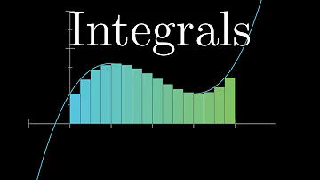 20:46
20:46
 4:56
4:56
 6:04
6:04
 3:38
3:38
 38:32
38:32
 8:20
8:20
 5:05
5:05
 4:11
4:11
 10:18
10:18
 34:06
34:06


